DJR-MCP Finder: AI-assisted structural biology for virus evolution
On 30 July 2026, I published the first formal release of DJR-MCP Finder v0.1 on GitHub. The software release is v0.1; the model shipped with it is Model V0. The mixed nominee discussed later remains an experimental candidate.
DJR-MCP Finder is a protein classifier for viral evolution research. It accepts protein FASTA sequences and searches for candidate major capsid proteins that may adopt the double-jelly-roll (DJR) fold and be associated with viral morphogenesis. The project was developed in the context of DJR-MCP lineages within Varidnaviria; it does not claim that every member of the realm uses a DJR-MCP.
Here I describe why I built the tool, the decisions I struggled with, and my experience working with Codex.
Why look for DJR-MCPs?
Major capsid proteins (MCPs) are central components of the capsids built by many viruses, predominantly double-stranded DNA viruses in this context. In viruses whose MCPs adopt the DJR fold, these proteins also provide important clues for studying viral morphogenesis, genome annotation, and deep evolutionary relationships.
The difficulty is that sequence similarity among distantly related DJR-MCPs can be very low. A search based only on existing annotations or high sequence similarity can therefore miss distantly related candidates.
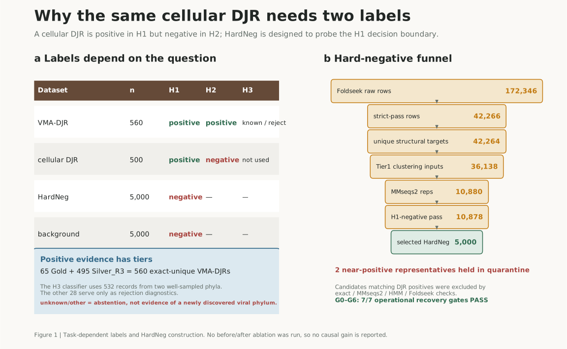
Cellular organisms also encode DJR proteins. Finding that fold alone is therefore insufficient to identify a protein as a viral MCP.
DJR-MCP Finder screens candidates, leaving the final identification to the user:
Reduce a large protein collection to a manageable candidate list with explicit evidence limits, so that structure, genomic context, and virological evidence can be examined next.
I therefore divided the problem into three tasks:
- H1: determine whether a protein has a DJR fold;
- H2: among DJR proteins, determine whether it is associated with viral morphogenesis;
- H3: attempt to assign it to one of two known viral phyla with enough labeled examples.
When the evidence for H3 is insufficient, the tool returns unknown/other. This is an abstention from a forced assignment, not evidence for a newly discovered viral phylum.
Hard negatives: easy negatives are not enough
If every H1 negative were an ordinary protein with little resemblance to DJR proteins, the model might score well using protein length, composition, or database source alone. That would tell me little about its ability to distinguish similar structures, so I built a separate set of structurally similar hard negatives.
The process began with 172,346 Foldseek search records. After quality filtering, deduplication, and MMseqs2 clustering, I used sequence, HMM, and structure checks to exclude candidates that still matched the DJR positives. I then selected 5,000 HardNeg representatives.
Two representatives were too close to the positive set. I placed them in quarantine and excluded them from training.
I use this set to check whether proteins supported as H1 negatives by sequence, HMM, and structure checks are still misclassified because they resemble DJRs.
I did not run a directly comparable before-and-after ablation, so I do not attribute a numerical performance gain to the hard-negative set. What I can verify is that rerunning the workflow from the frozen inputs reproduces the same representatives and final outputs, and that the exclusion rules and G0–G6 recovery gates are auditable. The project does not claim that every raw intermediate file was retained or reproduced byte for byte.
Split by component, not by sequence
Two protein records may be non-identical yet still belong to the same family or originate from the same upstream cluster.
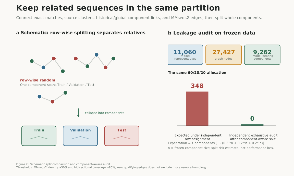
If each row is assigned independently to training, validation, and test partitions, the test set may contain close relatives of training examples. The resulting score can look excellent while overstating generalization.
To reduce this form of leakage, I first built a relation graph that connected records sharing any of the following:
- an identical normalized sequence;
- the same source cluster;
- a known historical or global component relationship;
- an MMseqs2 relationship with at least 30% identity and at least 80% coverage in both directions.
Each connected component in this graph became a relation component. All sequences in a component were assigned to the same partition.
The 11,060 modeling records formed 9,262 components containing at least one modeling record. Using the frozen component sizes, a row-wise random 60/20/20 split would be expected to split about 348 components across two or more partitions.
After the component-aware split, an independent workflow searched all three pairs of partitions. It found no exact duplicate sequences, no overlapping components, and no residual relationships that met the prespecified identity and coverage thresholds.
These checks document which relationships were isolated and the thresholds and procedures used to check them. Remote homologs below 30% identity may still remain across partitions.
Model selection cannot stop at the top score
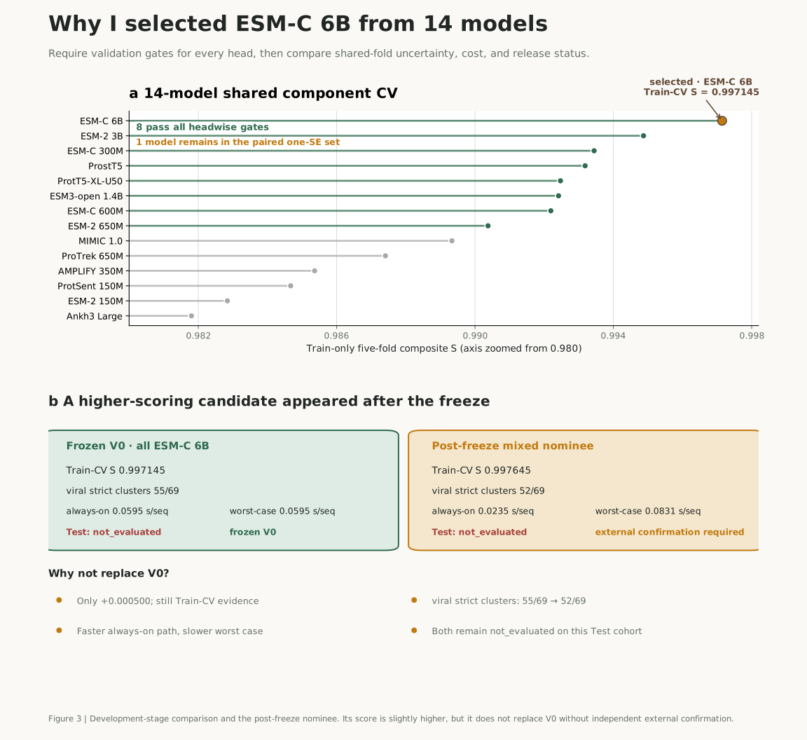
I compared 14 protein representation models using one fixed five-fold component assignment within the training partition.
Each model first had to pass a prespecified validation criterion for every task. The remaining models were then compared with a paired one-standard-error comparison across the same folds. Eight models passed every validation gate, but only ESM-C 6B remained in the one-standard-error set. I therefore froze it as Model V0.
These development scores come from Train-CV, not from the test set.
During this comparison, I found that sigmoid-transformed scores for one ESM-2 650M run had saturated to exact zeros and ones, producing an average precision (AP) of about 0.857. Recomputing AP from the corresponding raw decision scores, which retained ranking information, gave about 0.998 for the same run. The difference came from the metric input; the model had not changed.
That mistake showed me why I need to check the metric contract during model selection: what input each score takes and how it is calculated.
A slightly higher score is not enough to replace a frozen model
After freezing Model V0, I obtained a mixed-model candidate, referred to here as the mixed nominee, with a slightly higher composite score.
Its Train-CV score was about 0.0005 higher than V0’s, but it performed worse in the viral strict-cluster diagnostic, an internal post-freeze check, and had a slower worst-case inference path. I recorded it as recommended_for_external_confirmation and kept the frozen choice.
As I continued experimenting, I applied the existing release rules to new candidates instead of revising the selection with each change in rank.
not_evaluated can be a meaningful result
The project retains a protected test set containing 2,214 records.
This test set had already been opened for an earlier ESM-2 650M model. The subsequently selected ESM-C 6B model and the mixed nominee were not evaluated on it, so their model-level evaluation status remains not_evaluated.
I chose not to reopen the old test set. The next independent evaluation will require a new external lockbox separated from the existing source components.
Previously, I might have wanted to fill in the missing test metrics. This time I kept not_evaluated to record that these models had not undergone that evaluation and that I had not reused the old test set to obtain more attractive scores.
What Codex helped me accelerate
In the past, I usually used AI to solve isolated coding problems. In this project, I worked with Codex continuously in the same repository for the first time.
I used Codex to:
- draft and revise scripts;
- run tests and organize logs;
- compare intermediate results;
- expand literature-search terms;
- inspect citations, data leakage, and metric implementations;
- turn complex steps into review checklists.
At the start of each iteration, I defined the scientific question and constraints.
I checked the agent’s literature suggestions, labeling proposals, and methodological options myself. To decide whether a record met the Gold or Silver criteria and should be included, I went back to the original papers, figures, and database records. Once a rule was implemented, I reviewed diffs, logs, frozen files, and key artifacts, then revised and reran the analysis when I found a problem.
Codex let me work on literature search, implementation, testing, and review in parallel and find inconsistencies between them sooner. I still had to judge which results I could trust.
Based on my development records and recollection, the initial design through to the first completed benchmark took about two months. It would probably have taken longer without this collaboration. I remained responsible for the dataset boundaries, the biological evidence, and the final conclusions.
Reflections
1. An AI4S project starts with the right problem decomposition
A DJR fold is useful structural evidence, but it is not equivalent to viral identity. The existence of cellular DJRs forced me to separate H1 from H2. It also reinforced that model output must still be interpreted alongside structure, genomic context, and virological evidence.
2. Data and labels often matter more than the model
Much of the work went into collecting examples, validating Silver positives, constructing negative sets, and selecting representative sequences.
Protein language models provide useful representations, but interpreting their scores still depends on how the positive and negative classes were defined and whether close relatives of training records leaked into the test set.
3. In this project, protein language models did not replace traditional homology search
This benchmark did not give me evidence that protein language models dramatically outperform conventional sequence alignment or profile-HMM methods for homolog detection. The 14-model benchmark compared different protein-language-model representations; it was not a strict head-to-head comparison with MMseqs2 or HMM-based search. This is therefore a methodological judgment from the development process, not a quantitative claim about relative performance.
Traditional methods still provide interpretable alignments, explicit thresholds, and traceable hit relationships. Protein language models can help rank candidates when sequence similarity is weak and the classification boundary is complex. In practice, I use the two approaches to cross-check each other.
4. Preserving the limits of the evidence matters more than filling every cell
I kept several unresolved states in the results: quarantine for ambiguous examples, unknown/other for classifications with insufficient evidence, and not_evaluated for models without an independent evaluation. The table has gaps, but readers can see which judgments still need evidence.